
📌 Intro
MNIST 데이터 셋에 이어 FER2013데이터 셋을 이용하여 표정을 통해 감정인식 분류기를 만들어보자.
📌 Dataset FER2013
Overview
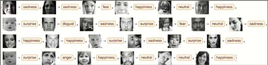
Label은 7개로 0=Angry, 1=Disgust, 2=Fear, 3=Happy, 4=Sad, 5=Surprise, 6=Neutral로 매핑되어 있다.
Image는 FER2013 이미지이고 48 x 48 x 1의 Shape을 가지고 있다.
MNIST를 사용할 때는 keras에 내장되어 있는 데이터 셋을 로드해서 사용했었지만, FER2013 데이터 셋은 keras에 내장되어 있지 않기 때문에 .csv파일을 다운받아 사용해야 한다.
Details
Challenges in Representation Learning: Facial Expression Recognition Challenge | Kaggle
www.kaggle.com
위 링크에서 fer2013.tar.gz를 다운 받고 압축 파일 내에 있는 fer2013.csv파일을 사용할 것이다.(회원가입을 해야만 다운 받을 수 있는 것 같다.)
fer2013.csv파일의 형태를 보면 다음과 같다.

- Emotion : 감정
- 0 = Angry
- 1 = Disgust
- 2 = Fear
- 3 = Happy
- 4 = Sad
- 5 = Surprise
- 6 = Neutral
- Pixels : 48 x 48 x 1 이미지
- Usage : 사용용도
- Training - 트레이닝
- PrivateTest - Validation
- PublicTest - 테스트
📌 전체 코드
import csv
import numpy as np
import pandas as pd
import matplotlib.pyplot as plt

from tensorflow.keras.models import Sequential
from tensorflow.keras.layers import Dense, Dropout, Activation, Flatten
from tensorflow.keras.layers import Conv2D, MaxPooling2D, BatchNormalization
from tensorflow.keras.losses import categorical_crossentropy
from tensorflow.keras.optimizers import Adam
from tensorflow.keras.regularizers import l2
from sklearn.model_selection import train_test_split

# 1. 데이터 셋 경로
fer2013_dataset_file_path = 'fer2013.csv'

train_images = []
train_labels = []

val_images = []
val_labels = []

test_images = []
test_labels = []

# 2. 파일로부터 데이터 읽어와 전처리
with open(fer2013_dataset_file_path) as csv_file:
    csv_reader = csv.reader(csv_file, delimiter=',')
    for row_id, row in enumerate(csv_reader):
        # 첫 번째 행 pass
        if row_id == 0:
            continue

        # 정답 레이블만 1로 생성
        label = np.zeros(7)
        label[int(row[0])] = 1

        image = list(map(int, row[1].split(' ')))

        # 분류
        if row[2] == 'Training':
            train_labels.append(label)
            train_images.append(image)
        elif row[2] == 'PublicTest':
            test_labels.append(label)
            test_images.append(image)
        elif row[2] == 'PrivateTest':
            val_labels.append(label)
            val_images.append(image)

train_labels = np.asarray(train_labels, dtype=np.float32)
train_images = np.asarray(train_images, dtype=np.float32).reshape(-1, 48, 48, 1)

val_labels = np.asarray(val_labels, dtype=np.float32)
val_images = np.asarray(val_images, dtype=np.float32).reshape(-1, 48, 48, 1)

test_labels = np.asarray(test_labels, dtype=np.float32)
test_images = np.asarray(test_images, dtype=np.float32).reshape(-1, 48, 48, 1)

# 3. 데이터 shape확인
print('Train images:', train_images.shape)
print('Train labels:', train_labels.shape)

print('Val images:', val_images.shape)
print('Val labels:', val_labels.shape)

print('Test images:', test_images.shape)
print('Test labels:', test_labels.shape)

# 4. normalization
train_images /= 255
val_images /= 255
test_images /= 255

emotions = {
    0: 'Angry',
    1: 'Disgust',
    2: 'Fear',
    3: 'Happy',
    4: 'Sad',
    5: 'Surprise',
    6: 'Neutral'
}

# 5. sample 데이터 확인
index = 0
print('Label array:', train_labels[index], '\nLabel:', np.argmax(train_labels[index]),
      '\nEmotion:', emotions[np.argmax(train_labels[index])],
      '\nImage shape:', train_images[index].shape)
plt.imshow(train_images[index].reshape(48, 48), cmap='gray')
plt.show()

# 6. 모델 구성
input_shape = (48, 48, 1)
num_labels = 7

num_features = 64

model = Sequential()

model.add(Conv2D(32, kernel_size=(3,3), input_shape=input_shape, activation='relu'))

model.add(Conv2D(32, kernel_size=(3,3), activation='relu'))
model.add(BatchNormalization())
model.add(MaxPooling2D(pool_size=(2, 2), strides=(2, 2)))
model.add(Dropout(0.5))

model.add(Flatten())

model.add(Dense(1000, activation='relu'))
model.add(Dropout(0.4))
model.add(Dense(num_labels, activation='softmax'))

model.summary()

# 7. 모델 컴파일 및 학습
batch_size = 512
epochs = 10

# adam과 categorical crossentropy loss를 이용하여 모델 컴파일
model.compile(loss=categorical_crossentropy,
              optimizer=Adam(learning_rate=0.001, beta_1=0.9, beta_2=0.999, epsilon=1e-7),
              metrics=['accuracy'])

# 모델 학습
train_history = model.fit(
    train_images, train_labels,
    batch_size=batch_size,
    epochs=epochs,
    validation_data=(val_images, val_labels),
    verbose=1)

# 8. 정확도 확인
loss, accuracy = model.evaluate(test_images, test_labels, verbose=1)
print('Loss:', loss, '\nAccuracy:', accuracy * 100, '%')📌 코드 설명
1. 데이터 셋 경로
fer2013.csv파일을 읽어올 수 있도록 path를 저장해둔다.
2. 파일로부터 데이터 읽어와 전처리
csv파일은 앞서 살펴본 것 처럼 컬럼별로 다른 정보가 들어가 있기 때문에 데이터를 알맞게 사용할 수 있도록 전처리가 필요하다.
첫 번째 행은 emotion, pixels, usage가 적혀있기 때문에 넘어가고 그 다음 행의 데이터부터 사용한다.
첫 번째 컬럼의 데이터를 이용하여 7개의 레이블 중 정답 레이블을 만든다. 만약 0번이 들어있었다면 정답 레이블은[1, 0, 0, 0, 0, 0. 0]이 될 것이다.
두 번째 컬럼의 데이터를 이용하여 이미지 리스트를 만들어준다. 이는 reshape()을 통해 48 x 48 x 1의 Shape으로 바꿔줄 것이다.
세 번째 컬럼의 데이터를 이용하여 앞에서 가공한 데이터를 Training, Validation, Test로 분류한다.
3. 데이터 shape확인
전처리해준 데이터의 Shape을 확인하면 다음과 같다.

training 데이터 28709장, validation 데이터 3589장, test 데이터 3589장으로 구성되어 있다.
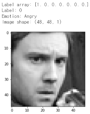
5. sample 데이터 확인
훈련 데이터의 첫 번째 데이터를 확인해보면 다음과 같다. (그런데 저 얼굴이 화난 얼굴인지는 잘 모르겠다)
6. 모델 구성

7. 모델 컴파일 및 학습
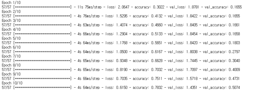
모델이 좀 크기 때문에 GPU가 있는 환경에서 학습을 진행하는 것을 추천한다.
8. 정확도 확인

약 50%정도의 정확도가 나오는 것을 확인하였다.
📌 정리
fer2013 데이터를 이용하여 감정인식 분류기를 만들어봤다. 현재 만든 모델은 정확도가 50%정도 되기 때문에 모델의 수정이 필요하다. 후에 더 성능이 좋은 모델을 만들어 정확도를 높이는 작업을 진행해보면 좋을 것 같다.
fer2013데이터는 아마 Kaggle에 회원가입을 해야 받을 수 있는 것으로 보여서 이 글을 보고 따라하는 분이 계신다면 그 부분에서 어려움이나 귀찮음을 느낄 수 있다고 생각된다. 필자가 데이터를 같이 올리면 편하겠지만 문제가 되는지 여부를 알지 못하여 쉽게 올리지 못하겠다. (이 부분은 양해해주시면 감사하겠습니다.)
사실 MNIST 데이터를 다루는 내용은 너무 쉽게 접할 수 있다. 그래도 감정 인식 모델을 만드는 내용은 그보다 적다고 생각되기 때문에 공부하는 목적과 다른 사람들에게도 도움이 되었으면 좋겠다는 생각에 정리를 시작했고, 그 목적이 이루어졌음 좋겠다.